
Poisson's equation
In mathematics, Poisson's equation is a partial differential equation with broad utility in electrostatics, mechanical engineering and theoretical physics. It is named after the French mathematician, geometer and physicist Siméon-Denis Poisson. The Poisson equation is

where Δ is the Laplace operator, and f and φ are real or complex-valued functions on a manifold. When the manifold is Euclidean space, the Laplace operator is often denoted as  and so Poisson's equation is frequently written as
and so Poisson's equation is frequently written as
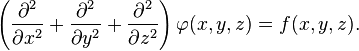
In three-dimensional Cartesian coordinates, it takes the form
For vanishing f, this equation becomes Laplace's equation

The Poisson equation may be solved using a Green's function; a general exposition of the Green's function for the Poisson equation is given in the article on the screened Poisson equation. There are various methods for numerical solution. The relaxation method, an iterative algorithm, is one example.
Electrostatics
One of the cornerstones of electrostatics is the posing and solving of problems that are described by the Poisson equation. Finding φ for some given f is an important practical problem, since this is the usual way to find the electric potential for a given charge distribution.
The derivation of Poisson's equation in electrostatics follows. SI units are used and Euclidean space is assumed.
Starting with Gauss' law for electricity (also part of Maxwell's equations) in a differential control volume, we have:

 is the divergence operator.
 is the electric displacement field.
 is the free charge density (describing charges brought from outside).
Assuming the medium is linear, isotropic, and homogeneous (see polarization density), then:

 is the permittivity of the medium.
 is the electric field.
By substitution and division, we have:

In the absence of a changing magnetic field,  , Faraday's law of induction gives:
, Faraday's law of induction gives:
 is the curl operator.
- t is time.
Since the curl of the electric field is zero, it is defined by a scalar electric potential field,  (see Helmholtz decomposition).
(see Helmholtz decomposition).
Eliminating by substitution, we have a form of the Poisson equation:
by substitution, we have a form of the Poisson equation:
Solving Poisson's equation for the potential requires knowing the charge density distribution. If the charge density is zero, then Laplace's equation results. If the charge density follows a Boltzmann distribution, then the Poisson-Boltzmann equation results. The Poisson-Boltzmann equation plays a role in the development of the Debye-Hückel theory of dilute electrolyte solutions.
(Note: Although the above discussion assumes that the magnetic field is not varying in time, the same Poisson equation arises even if it does vary in time, as long as the Coulomb gauge is used. However, in this more general context, computing is no longer sufficient to calculate , since the latter also depends on the magnetic vector potential, which must be independently computed.)
is no longer sufficient to calculate , since the latter also depends on the magnetic vector potential, which must be independently computed.)Potential of a Gaussian charge density
If there is a static spherically symmetric Gaussian charge density ρf(r):

where Q is the total charge, then the solution φ (r) of Poisson's equation,
 ,
,
is given by

where erf(x) is the error function. This solution can be checked explicitly by evaluating  . Note that, for r much greater than σ, the erf function approaches unity and the potential φ (r) approaches the point charge
 , as one would expect. Furthermore the erf function approaches 1 extremely quickly as its argument increases; in practice for r > 3σ the relative error is smaller than one part in a thousand.
. Note that, for r much greater than σ, the erf function approaches unity and the potential φ (r) approaches the point charge, as one would expect. Furthermore the erf function approaches 1 extremely quickly as its argument increases; in practice for r > 3σ the relative error is smaller than one part in a thousand.